MITライセンスで配布されているsimcirJSでデジタル基礎で学ぶ回路を再現しました.
カテゴリー: 講義
講義資料
物理情報数学B,バイオシステムおよび実験レポートのグラフについて,Pythonのプログラムの例へのリンクのページを作成しました.1, 2, 3年生の皆さんへのページにリンクがあります.
特異値分解
物理情報数学Bで扱った行列AをA=UΣVTに特異値分解します.
#
import numpy as np
import matplotlib.pyplot as plt
A = np.array([[2, 2], [-1, 2]])
U, S, V = np.linalg.svd(A) # V^TがVに入ることに注意する
print("特異値分解")
print("U")
print(U)
print("S")
print(S)
print("V")
print(V)
print("USV^T")
S2 = np.eye(2)*S
#
plt.figure(figsize=(5, 5))
plt.xlim([-3, 3])
plt.ylim([-3, 3])
plt.xlabel('x1')
plt.ylabel('x2')
print(np.dot(np.dot(U, S2), V))
#
theta = np.arange(0, 361, 3)
uc = np.array([np.cos(theta/180*np.pi), np.sin(theta/180*np.pi)])
#
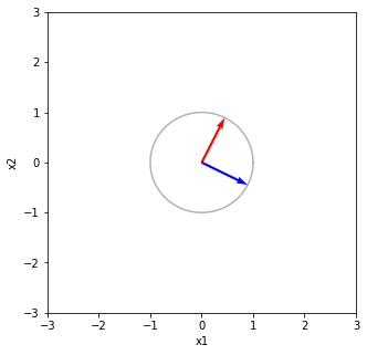
print("Vの列ベクトルと単位円")
plt.plot(uc[0,:], uc[1,:], color='black', alpha=0.3)
plt.quiver(0, 0, V[0, 0], V[0, 1], angles="xy", scale_units='xy', scale=1, color='red')
plt.quiver(0, 0, V[1, 0], V[1, 1], angles="xy", scale_units='xy', scale=1, color='blue')
plt.show()
x1 = np.dot(V, V.T)
c1 = np.dot(V, uc)
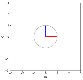
print("Vの列をV^Tで写像する V^TV 回転と鏡映")
print(x1)
plt.figure(figsize=(5, 5))
plt.xlim([-3, 3])
plt.ylim([-3, 3])
plt.xlabel('x1')
plt.ylabel('x2')
plt.plot(c1[0,:], c1[1,:], color='black', alpha=0.3)
plt.quiver(0, 0, x1[0, 0], x1[1, 0], angles="xy", scale_units='xy', scale=1, color='red')
plt.quiver(0, 0, x1[0, 1], x1[1, 1], angles="xy", scale_units='xy', scale=1, color='blue')
plt.show()
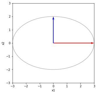
print("それをシグマで写像する ΣV^TV 軸方向に拡大・縮小(特異値倍)する")
x2 = np.dot(S2, x1 )
c2 = np.dot(S2, c1)
print(x2)
plt.figure(figsize=(5, 5))
plt.xlim([-3, 3])
plt.ylim([-3, 3])
plt.xlabel('x1')
plt.ylabel('x2')
plt.plot(c2[0,:], c2[1,:], color='black', alpha=0.3)
plt.quiver(0, 0, x2[0, 0], x2[1, 0], angles="xy", scale_units='xy', scale=1, color='red')
plt.quiver(0, 0, x2[0, 1], x2[1, 1], angles="xy", scale_units='xy', scale=1, color='blue')
plt.show()
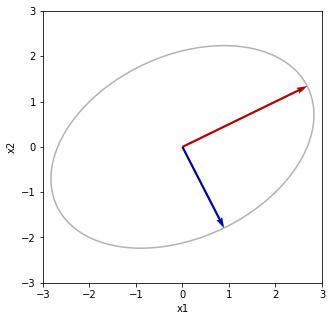
print("最後にUで写像する UΣV^TV 回転と鏡映")
print("u1とu2のσ1倍とσ2倍にそれぞれ重なる")
x3 = np.dot(U, x2)
c3 = np.dot(U, c2)
print(x3)
plt.figure(figsize=(5, 5))
plt.xlim([-3, 3])
plt.ylim([-3, 3])
plt.xlabel('x1')
plt.ylabel('x2')
plt.plot(c3[0,:], c3[1,:], color='black', alpha=0.3)
plt.quiver(0, 0, x3[0, 0], x3[1, 0], angles="xy", scale_units='xy', scale=1, color='red')
plt.quiver(0, 0, x3[0, 1], x3[1, 1], angles="xy", scale_units='xy', scale=1, color='blue')
plt.quiver(0, 0, S[0]*U[0, 0], S[0]*U[1, 0], angles="xy", scale_units='xy', scale=1, color='black', alpha=0.3)
plt.quiver(0, 0, S[1]*U[0, 1], S[1]*U[1, 1], angles="xy", scale_units='xy', scale=1, color='black', alpha=0.3)
plt.show()
特異値分解
U
[[ 0.89442719  0.4472136 ]
 [ 0.4472136  -0.89442719]]
S
[3. 2.]
V
[[ 0.4472136   0.89442719]
 [ 0.89442719 -0.4472136 ]]
USV^T
[[ 2.  2.]
 [-1.  2.]]
Vの列ベクトルと単位円
Vの列をV^Tで写像する V^TV 回転と鏡映
[[ 1.00000000e+00 -2.43158597e-17]
 [-2.43158597e-17  1.00000000e+00]]
それをシグマで写像する ΣV^TV 軸方向に拡大・縮小(特異値倍)する
 [[ 3.00000000e+00 -7.29475792e-17]
  [-4.86317195e-17  2.00000000e+00]]
最後にUで写像する UΣV^TV 回転と鏡映 u1とu2のσ1倍とσ2倍にそれぞれ重なる
 [[ 2.68328157  0.89442719]
  [ 1.34164079 -1.78885438]]
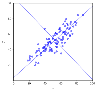
主成分分析
物理情報数学Bで説明していている対称行列が出てくる例です.固有ベクトルへの射影も関係します.
#
# 主成分分析
#
import numpy as np
import matplotlib.pyplot as plt
from sklearn.decomposition import PCA
N = 100
d = 16
x = 50 + np.random.randn(N) * d
y = 0.8 * x + np.random.randn(N) * d * 0.5 + 10
plt.figure(figsize=(5, 5))
plt.xlim([0, 100])
plt.ylim([0, 100])
plt.xlabel('x')
plt.ylabel('y')
plt.scatter(x, y, color='blue', alpha=0.5)
features = np.vstack([x, y]).T
features2 = features.copy()
ave = np.average(features,0)
print("平均")
print(ave)
features = features - ave
cv = np.dot(features.T, features) / (N - 1)
print("共分散行列")
print(cv)
W, v = np.linalg.eig(cv)
print("共分散行列の固有ベクトルを列にもつ行列")
print("{0}".format(v))
print("固有ベクトル")
print("{0}".format(v[:,0].reshape(2,1)))
print("固有ベクトル")
print("{0}".format(v[:,1].reshape(2,1)))
print("共分散行列の固有値:{0}".format(W))
# 寄与率は固有値/(固有値の総和)
p = np.trace(cv)
print("寄与率1: {0}, 2: {1}".format(W[0]/p, W[1]/p))
# 固有値の大きい順にソート
ind = np.argsort(W)[::-1]
sortedW = np.sort(W)[::-1]
sortedv = v[:,ind]
# 固有ベクトル方向の直線
plt.plot(np.array([0, 100]), np.array([sortedv[1,0]/sortedv[0,0]*(0 - ave[0])+ave[1], sortedv[1,0]/sortedv[0,0]*(100 - ave[0])+ave[1]]), color='blue', alpha=0.5)
plt.plot(np.array([0, 100]), np.array([sortedv[1,1]/sortedv[0,1]*(0 - ave[0])+ave[1], sortedv[1,1]/sortedv[0,1]*(100 - ave[0])+ave[1]]), color='blue', alpha=0.5)
#
t1 = np.zeros([2, N])
# 固有ベクトル方向に射影する
#p1 = v[:,0].reshape(2,1)
#p2 = v[:,1].reshape(2,1)
#for i in range(N):
# t1[0, i] = np.dot(p1.T, (features.T[:,i]).reshape(2,1)) # 射影するベクトルは単位ベクトルなので2乗ノルムの2乗で割る必要なし
# t1[1, i] = np.dot(p2.T, (features.T[:,i]).reshape(2,1))
t1 = np.dot(sortedv.T, features.T)
#
plt.figure(figsize=(5, 5))
plt.xlim([-70, 70])
plt.ylim([-70, 70])
plt.xlabel('p1')
plt.ylabel('p2')
plt.scatter(t1[0,:], t1[1,:], color='red', alpha=0.5)
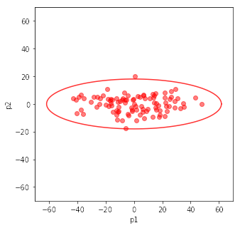
# 3σの楕円
theta = np.arange(0, 361, 3)
X = np.cos(theta/180*np.pi) * np.sqrt(sortedW[0]) * 3
Y = np.sin(theta/180*np.pi) * np.sqrt(sortedW[1]) * 3
plt.plot(X, Y, color='red', alpha=0.8)
plt.show()
#
#
print("主成分分析のライブラリを使う")
pca = PCA(n_components=2)
pca.fit(features2)
print("components")
print("{0}".format(pca.components_))
print("mean={0}".format(pca.mean_))
print("covariance")
print("{0}".format(pca.get_covariance()))
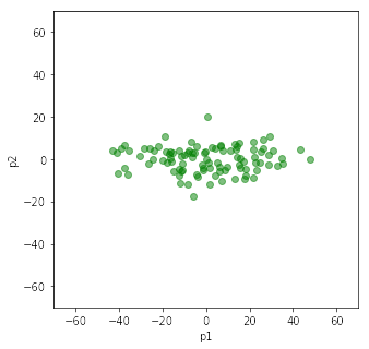
t2 = pca.fit_transform(features)
print("contribution")
print(pca.explained_variance_ratio_)
plt.figure(figsize=(5, 5))
plt.xlim([-70, 70])
plt.ylim([-70, 70])
plt.xlabel('p1')
plt.ylabel('p2')
plt.scatter(t2[:,0], t2[:,1], color='green', alpha=0.5)
print("固有ベクトルの符号が反転していると左右・上下に反転がある")
plt.show()
平均
[52.53235793 51.86342693]
共分散行列
[[244.04297958 193.42743647]
 [193.42743647 216.02097448]]
共分散行列の固有ベクトルを列にもつ行列
[[ 0.73220426 -0.6810851 ]
 [ 0.6810851   0.73220426]]
固有ベクトル
[[0.73220426]
 [0.6810851 ]]
固有ベクトル
[[-0.6810851 ]
 [ 0.73220426]]
共分散行列の固有値:[423.96619622  36.09775785]
寄与率1: 0.9215375220555805, 2: 0.07846247794441952
主成分分析のライブラリを使う
components
[[ 0.73220426  0.6810851 ]
 [-0.6810851   0.73220426]]
mean=[52.53235793 51.86342693]
covariance
[[244.04297958 193.42743647]
 [193.42743647 216.02097448]]
contribution
[0.92153752 0.07846248]
固有ベクトルの符号が反転していると左右・上下に反転がある
第1主成分は,固有値が最も大きい固有ベクトルの方向です.固有値が最も大きい方向は,データの散らばりが最も大きくなる方向です.これは次のように導くことができます.
ベクトル$\mathbf x_i$の平均は$\bar{\mathbf x}=\displaystyle\frac{1}{N}\sum_{i=1}^{N}\mathbf x_i$です.
今,データのベクトル$\mathbf x_i$をデータの散らばりが最も大きくなる方向のベクトル$\mathbf u_1$に射影することを考えます.このとき,$\mathbf u_1$を単位ベクトルにとります.$\mathbf x_i$を$\mathbf u_1$に射影すると$\mathbf x_i^T\mathbf u_1$になります.射影の分散は
$\sigma^2 = \displaystyle\frac{1}{N}\sum_{i=1}^{N}(\mathbf x_i^T\mathbf u_1 – \bar{\mathbf x}^T\mathbf u_1)^2 = \mathbf u_1^T S \mathbf u_1$です.
ここで
$S= \displaystyle\frac{1}{N}(\mathbf x_i – \bar{\mathbf x})(\mathbf x_i – \bar{\mathbf x})^T$です.
$\mathbf u_1^T S \mathbf u_1$を$\mathbf u_1^T\mathbf u_1=1$の条件の下で最大化します.これはラグランジェの未定乗数法を用いて
$\mathbf u_1^T S \mathbf u_1 – \lambda(\mathbf u_1^T\mathbf u_1 – 1)$
を最大化して解きます.$\mathbf u_1$で微分すると
$S\mathbf u_1 – \lambda \mathbf u_1=0$
になります.つまり$S\mathbf u_1 = \lambda \mathbf u_1$ですから,$\mathbf u_1$は行列$S$の固有ベクトルです.
この式に左から$\mathbf u_1^T$をかけると$\mathbf u_1^T S \mathbf u_1 = \lambda$となり,データ$\mathbf x_i$の射影の分散は固有値です.また,それを最大にするものは最大の固有値になります.
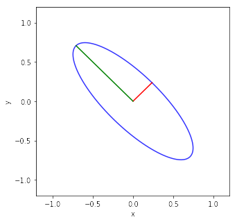
傾いた楕円の式
物理情報数学Bで対称行列の応用例として取り上げている傾いた楕円の式の説明です.
$5x^2 + 8xy + 5y^2 = 1$
の式を行列で表すと
$\left[\begin{array}{cc}x & y\end{array}\right]\left[\begin{array}{cc}5 & 4\\ 4 & 5\end{array}\right]\left[\begin{array}{c}x\\ y\end{array}\right]=1$
になる.
行列を$A$と置くと,$A$の固有ベクトル(正規化されたもの)を列に持つ行列$Q$を用いて$A=Q\Lambda Q^T$と表せる.行列$A$は固有値として9と1を持つ.固有値が9のとき固有ベクトルは$[1\ 1]^T$である.固有値が1のとき固有ベクトルは$[1\ -1]^T$である.固有ベクトルの大きさは$\sqrt{2}$であるので
$\left[\begin{array}{cc}x & y\end{array}\right]\displaystyle\frac{1}{\sqrt{2}}\left[\begin{array}{rr}1 & 1\\ 1 & -1\end{array}\right]\left[\begin{array}{cc}9 & 0\\ 0 & 1\end{array}\right]\frac{1}{\sqrt{2}}\left[\begin{array}{rr}1 & 1\\ 1 & -1\end{array}\right]\left[\begin{array}{c}x\\ y\end{array}\right]=1$
となる.
この式は
$9\left(\displaystyle\frac{x+y}{\sqrt{2}}\right)^2 + 1\left(\displaystyle\frac{x-y}{\sqrt{2}}\right)^2=1$
と表せる.括弧内を$X$と$Y$と置くと,
$9X^2+Y^2=1$
の楕円の式になる.楕円の短半径は1/3で長半径は1になる.これらは,固有値の逆数の平方根である.
import numpy as np
import matplotlib.pyplot as plt
import numpy.linalg as LA

#
# 5x^2 + 8xy + 5y^2 = 1
# 9X^2 + y^2 = 1
# X = (x + y)/sqrt(2)
# Y = (x - y) /sqrt(2)
#
theta = np.arange(0, 361, 3)
X = np.cos(theta/180*np.pi)/3
Y = np.sin(theta/180*np.pi)
x = (X+Y)/np.sqrt(2)
y = (X-Y)/np.sqrt(2)
plt.figure(figsize=(5, 5))
plt.xlim([-1.2, 1.2])
plt.ylim([-1.2, 1.2])
plt.xlabel('x')
plt.ylabel('y')
plt.plot(x, y, color='blue', alpha=0.8)
#
A = np.array([[5, 4], [4, 5]])
w,v = LA.eig(A)
print('固有値')
print(w)
print('固有ベクトル')
print(v)
# 固有値の逆数の平方根が長半径と短半径
# 固有ベクトルが軸方向
a = v[:,0].reshape(2, 1) / np.sqrt(w[0])
b = v[:,1].reshape(2 ,1) / np.sqrt(w[1])
plt.plot(np.array([0, a[0]]), np.array([0, a[1]]), color='red')
plt.plot(np.array([0, b[0]]), np.array([0, b[1]]), color='green')
plt.show()
固有値
[9. 1.]
固有ベクトル
[[ 0.70710678 -0.70710678]
 [ 0.70710678  0.70710678]]
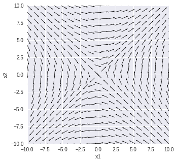
固有値・固有ベクトルと行列微分方程式
Google Colaboratoryが重いので結果だけ載せます.
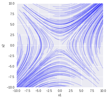
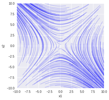
$\displaystyle\frac{dx_1(t)}{dt} = x_2(t)$
$\displaystyle\frac{dx_2(t)}{dt}=x_1(t)$
で固有値の1つが正で1つが負の場合
import numpy as np
import matplotlib.pyplot as plt
import numpy.linalg as LA
import random

A = np.array([[0, 1], [1, 0]])
w, v = LA.eig(A)
print('固有値')
print(w)
print('固有ベクトル')
print(v)
x10 = 4
x20 = 2
t = np.arange(0.0, 2.0, 0.1)
x10 = [random.uniform(-10, 10) for i in range(300)]
x20 = [random.uniform(-10, 10) for i in range(300)]

N = 22
x = np.linspace(-10,  10,  N)
y = np.linspace(-10,  10,  N)
(xm, ym) = np.meshgrid(x, y)
dxdt = ym
dydt = xm
norm = (np.sqrt(dxdt**2 + dydt**2))
dxdt2 = dxdt/norm
dydt2 = dydt/norm
plt.figure(figsize=(5, 5))
plt.quiver(xm, ym, dxdt2, dydt2, angles='xy', scale_units='xy', scale=1)
plt.xlim([-10, 10])
plt.ylim([-10, 10])
plt.xlabel('x1')
plt.ylabel('x2')
plt.show()

# 解析解
plt.figure(figsize=(5, 5))
for i in range(300):
  c = LA.solve(v, np.array([x10[i], x20[i]]))
  xxa = c[0] * np.exp(w[0]*t) * v[:,0].reshape(2, 1) +c[1] * np.exp(w[1]*t) * v[:,1].reshape(2, 1)
  plt.plot(xxa[0,:], xxa[1,:], color='blue', alpha=0.2)
plt.xlim([-10, 10])
plt.ylim([-10, 10])
plt.xlabel('x1')
plt.ylabel('x2')
plt.show()
固有値
[ 1. -1.]
固有ベクトル
[[ 0.70710678 -0.70710678]
 [ 0.70710678  0.70710678]]
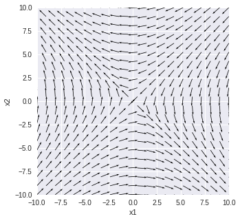
$\displaystyle\frac{dx_1(t)}{dt} = -x_2(t)$
$\displaystyle\frac{dx_2(t)}{dt}=-x_1(t)$
で固有値の1つが正で1つが負の場合
固有値
[ 1. -1.]
固有ベクトル
[[ 0.70710678  0.70710678]
 [-0.70710678  0.70710678]]
Pythonでバイオシステム
3年生秋学期後半の選択科目,バイオシステムで扱う内容の一部をPythonで実装したものです.keio IDが必要です.
Pythonで物理情報数学B
線形代数の計算をPythonのプログラムで表しました.keio IDが必要です.
Pythonでグラフ
Pythonで簡単なグラフを描くためのサンプルです.Google Colaboratoryを使います.keio IDが必要です.
餌と捕食者の関係
物理情報数学Bで,行列の累乗の応用例として,餌と捕食者の関係を表す行列差分方程式を説明しています.
「第[latex]k[/latex]年のイワシの数を[latex]x_1(k)[/latex],クジラの数を[latex]x_2(k)[/latex]とする.クジラがいないときの1年後のイワシの数を[latex]\alpha x_1(k)[/latex]とする.つまり,第[latex]k[/latex]年のイワシの数に比例して変化する.クジラに1年間に食べられるイワシの数を[latex]\beta x_2(k)[/latex]とする.つまり,クジラの数に比例するイワシが食べられる.イワシがいないときの1年後のクジラの数を[latex]\gamma x_2(k)[/latex]とする.また,イワシを食べて1年間に増加するクジラの数を[latex]\delta x_1(k)[/latex]とする.」
上記の関係を行列差分方程式で表すと
[latex]
\left[\begin{array}{c}x_1(k+1) \\x_2(k+2)\end{array}\right]
=
\left[\begin{array}{rr}\alpha & -\beta \\ \delta & \gamma\end{array}\right]
\left[\begin{array}{c}x_1(k) \\x_2(k)\end{array}\right]
[/latex]
になります.一般解は
[latex]\boldsymbol{x}(k) = \left[\begin{array}{rr}\alpha & -\beta \\ \delta & \gamma\end{array}\right]^k\boldsymbol{x}(0)[/latex]
になります.
この行列差分方程式を講義では手計算で解けるように,[latex]\alpha=1.5[/latex],[latex]\beta=0.25[/latex],[latex]\gamma=1.1[/latex],[latex]\delta=0.07[/latex]として解きます.しかし,この行列の固有値は1以上の実数が2つですので,餌と捕食者の数の変化に期待される振動的な振る舞いにはなりません.初期値のクジラの数が多いと,下図のようにイワシの数は減少に転じます.

餌と捕食者の関係のモデルとしては,ロトカ・ボルテラのモデルが知られています.このモデルでは,
[latex]
\displaystyle\frac{dx_1(t)}{dt} = \alpha x_1(t) – \beta x_1(t)x_2(t) \\
\displaystyle\frac{dx_2(t)}{dt} = \delta x_1(t)x_2(t) – \gamma x_2(t)
[/latex]
で表されます.非線形微分方程式ですから,[latex]x_1(t)[/latex]と[latex]x_2(t)[/latex]を解析的に求めることはできません.適当な値を代入して数値解を求めると,[latex]x_1(t)[/latex]と[latex]x_2(t)[/latex]が振動的な振る舞いをすることがわかります.
また,平衡点は[latex]dx_1(t)/dt=0[/latex]と[latex]dx_2(t)/dt=0[/latex]から,原点と[latex]x_1=\gamma/\delta[/latex],[latex]x_2=\alpha/\beta[/latex]にあります.平衡点近傍では,[latex]x_1(t)x_2(t)[/latex]の項が小さいので無視できると仮定すると,[latex](0, 0)[/latex]の平衡点近傍では,
[latex]
\displaystyle\frac{d}{dt}\left[\begin{array}{c}x_1(t) \\x_2(t)\end{array}\right]
=
\left[\begin{array}{rr}\alpha & 0 \\
0 & -\gamma\end{array}\right]
\left[\begin{array}{c}x_1(t) \\x_2(t)\end{array}\right]
[/latex]
となり,行列の固有値は実数で1つは正でもう1つは負です.したがって,[latex](0, 0)[/latex]は鞍点です.
また,もう1つの平衡点[latex](\gamma/\delta, \alpha/\beta)[/latex]の近傍では,[latex]x_1(t)[/latex]を[latex]x_1+\gamma/\delta[/latex],[latex]x_2(t)[/latex]を[latex]x_2+\alpha/\beta[/latex]とおいて,[latex]x_1(t)x_2(t)[/latex]の項が小さいので無視できると仮定すると
[latex]
\displaystyle\frac{d}{dt}\left[\begin{array}{c}x_1(t) \\x_2(t)\end{array}\right]
=
\left[\begin{array}{rr}0 & -\frac{\beta\gamma}{\delta} \\
\frac{\alpha\delta}{\beta} & 0\end{array}\right]
\left[\begin{array}{c}x_1(t) \\x_2(t)\end{array}\right]
[/latex]
と表されます.したがって,固有値が純虚数となり,振動する解になります.
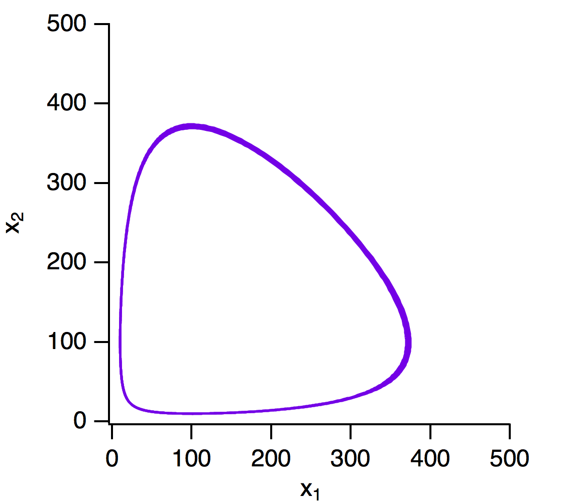
[latex]\alpha=10[/latex],[latex]\beta=0.1[/latex],[latex]\gamma=10[/latex],[latex]\delta=0.1[/latex]とし,[latex]x_1(0)=10[/latex]と[latex]x_2(0)=100[/latex] で数値解を求めると下図のようになります.上のパネルは[latex]x_1(t)[/latex]と[latex]x_2(t)[/latex]の時間発展です. 下のパネルは[latex]x_1(t)[/latex]と[latex]x_2(t)[/latex]の関係です.

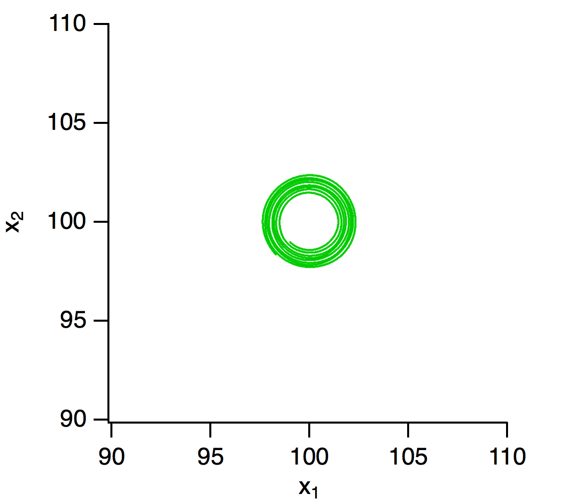
初期値を平衡点((100, 100))に近い点(99, 99)とすると下図のように円に近い軌道を描きます.
MATLABのコードです.
- lv.m
tspan = [0:0.001:5];
[t y] = ode45(@LotkaVolterra,tspan, [99 99]);
figure(1);
plot(t, y(:,1), 'b', t, y(:,2), 'r');
figure(2);
plot(y(:,1), y(:,2));
- LotkaVolterra.m
function dx = LotkaVolterra(t, x)
alpha = 10;
beta = 0.1;
gamma = 10;
delta = 0.1;
dx = zeros(2,1);
dx(1) = alpha * x(1) - beta * x(1) * x(2);
dx(2) = delta * x(1) * x(2) - gamma * x(2);
end