Google Colaboratoryが重いので結果だけ載せます.
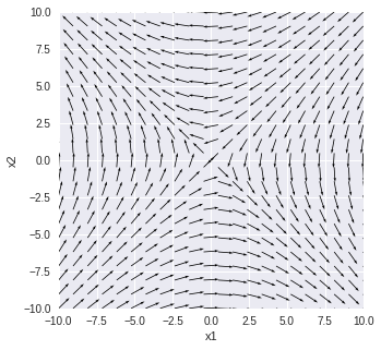
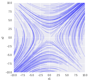
$\displaystyle\frac{dx_1(t)}{dt} = x_2(t)$
$\displaystyle\frac{dx_2(t)}{dt}=x_1(t)$
で固有値の1つが正で1つが負の場合
import numpy as np
import matplotlib.pyplot as plt
import numpy.linalg as LA
import random
A = np.array([[0, 1], [1, 0]])
w, v = LA.eig(A)
print('固有値')
print(w)
print('固有ベクトル')
print(v)
x10 = 4
x20 = 2
t = np.arange(0.0, 2.0, 0.1)
x10 = [random.uniform(-10, 10) for i in range(300)]
x20 = [random.uniform(-10, 10) for i in range(300)]
N = 22
x = np.linspace(-10, 10, N)
y = np.linspace(-10, 10, N)
(xm, ym) = np.meshgrid(x, y)
dxdt = ym
dydt = xm
norm = (np.sqrt(dxdt**2 + dydt**2))
dxdt2 = dxdt/norm
dydt2 = dydt/norm
plt.figure(figsize=(5, 5))
plt.quiver(xm, ym, dxdt2, dydt2, angles='xy', scale_units='xy', scale=1)
plt.xlim([-10, 10])
plt.ylim([-10, 10])
plt.xlabel('x1')
plt.ylabel('x2')
plt.show()
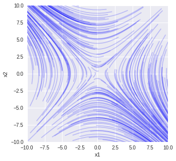
# 解析解
plt.figure(figsize=(5, 5))
for i in range(300):
c = LA.solve(v, np.array([x10[i], x20[i]]))
xxa = c[0] * np.exp(w[0]*t) * v[:,0].reshape(2, 1) +c[1] * np.exp(w[1]*t) * v[:,1].reshape(2, 1)
plt.plot(xxa[0,:], xxa[1,:], color='blue', alpha=0.2)
plt.xlim([-10, 10])
plt.ylim([-10, 10])
plt.xlabel('x1')
plt.ylabel('x2')
plt.show()
固有値
[ 1. -1.]
固有ベクトル
[[ 0.70710678 -0.70710678]
 [ 0.70710678  0.70710678]]
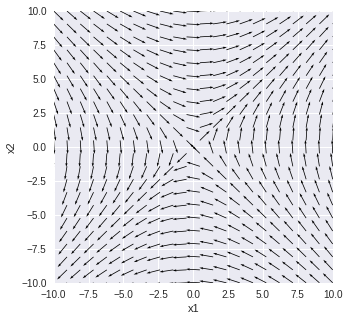
$\displaystyle\frac{dx_1(t)}{dt} = -x_2(t)$
$\displaystyle\frac{dx_2(t)}{dt}=-x_1(t)$
で固有値の1つが正で1つが負の場合
固有値
[ 1. -1.]
固有ベクトル
[[ 0.70710678  0.70710678]
 [-0.70710678  0.70710678]]