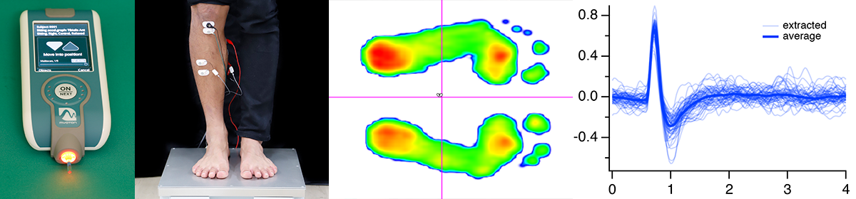
物理情報数学Bで説明していている対称行列が出てくる例です.固有ベクトルへの射影も関係します.
#
# 主成分分析
#
import numpy as np
import matplotlib.pyplot as plt
from sklearn.decomposition import PCA
N = 100
d = 16
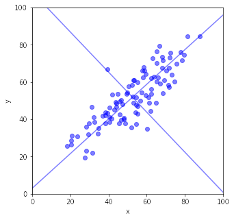
x = 50 + np.random.randn(N) * d
y = 0.8 * x + np.random.randn(N) * d * 0.5 + 10
plt.figure(figsize=(5, 5))
plt.xlim([0, 100])
plt.ylim([0, 100])
plt.xlabel('x')
plt.ylabel('y')
plt.scatter(x, y, color='blue', alpha=0.5)
features = np.vstack([x, y]).T
features2 = features.copy()
ave = np.average(features,0)
print("平均")
print(ave)
features = features - ave
cv = np.dot(features.T, features) / (N - 1)
print("共分散行列")
print(cv)
W, v = np.linalg.eig(cv)
print("共分散行列の固有ベクトルを列にもつ行列")
print("{0}".format(v))
print("固有ベクトル")
print("{0}".format(v[:,0].reshape(2,1)))
print("固有ベクトル")
print("{0}".format(v[:,1].reshape(2,1)))
print("共分散行列の固有値:{0}".format(W))
# 寄与率は固有値/(固有値の総和)
p = np.trace(cv)
print("寄与率1: {0}, 2: {1}".format(W[0]/p, W[1]/p))
# 固有値の大きい順にソート
ind = np.argsort(W)[::-1]
sortedW = np.sort(W)[::-1]
sortedv = v[:,ind]
# 固有ベクトル方向の直線
plt.plot(np.array([0, 100]), np.array([sortedv[1,0]/sortedv[0,0]*(0 - ave[0])+ave[1], sortedv[1,0]/sortedv[0,0]*(100 - ave[0])+ave[1]]), color='blue', alpha=0.5)
plt.plot(np.array([0, 100]), np.array([sortedv[1,1]/sortedv[0,1]*(0 - ave[0])+ave[1], sortedv[1,1]/sortedv[0,1]*(100 - ave[0])+ave[1]]), color='blue', alpha=0.5)
#
t1 = np.zeros([2, N])
# 固有ベクトル方向に射影する
#p1 = v[:,0].reshape(2,1)
#p2 = v[:,1].reshape(2,1)
#for i in range(N):
# t1[0, i] = np.dot(p1.T, (features.T[:,i]).reshape(2,1)) # 射影するベクトルは単位ベクトルなので2乗ノルムの2乗で割る必要なし
# t1[1, i] = np.dot(p2.T, (features.T[:,i]).reshape(2,1))
t1 = np.dot(sortedv.T, features.T)
#
plt.figure(figsize=(5, 5))
plt.xlim([-70, 70])
plt.ylim([-70, 70])
plt.xlabel('p1')
plt.ylabel('p2')
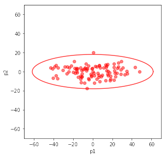
plt.scatter(t1[0,:], t1[1,:], color='red', alpha=0.5)
# 3σの楕円
theta = np.arange(0, 361, 3)
X = np.cos(theta/180*np.pi) * np.sqrt(sortedW[0]) * 3
Y = np.sin(theta/180*np.pi) * np.sqrt(sortedW[1]) * 3
plt.plot(X, Y, color='red', alpha=0.8)
plt.show()
#
#
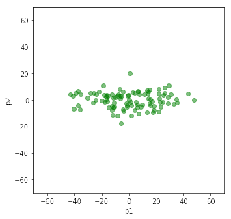
print("主成分分析のライブラリを使う")
pca = PCA(n_components=2)
pca.fit(features2)
print("components")
print("{0}".format(pca.components_))
print("mean={0}".format(pca.mean_))
print("covariance")
print("{0}".format(pca.get_covariance()))
t2 = pca.fit_transform(features)
print("contribution")
print(pca.explained_variance_ratio_)
plt.figure(figsize=(5, 5))
plt.xlim([-70, 70])
plt.ylim([-70, 70])
plt.xlabel('p1')
plt.ylabel('p2')
plt.scatter(t2[:,0], t2[:,1], color='green', alpha=0.5)
print("固有ベクトルの符号が反転していると左右・上下に反転がある")
plt.show()
平均
[52.53235793 51.86342693]
共分散行列
[[244.04297958 193.42743647]
 [193.42743647 216.02097448]]
共分散行列の固有ベクトルを列にもつ行列
[[ 0.73220426 -0.6810851 ]
 [ 0.6810851   0.73220426]]
固有ベクトル
[[0.73220426]
 [0.6810851 ]]
固有ベクトル
[[-0.6810851 ]
 [ 0.73220426]]
共分散行列の固有値:[423.96619622  36.09775785]
寄与率1: 0.9215375220555805, 2: 0.07846247794441952
主成分分析のライブラリを使う
components
[[ 0.73220426  0.6810851 ]
 [-0.6810851   0.73220426]]
mean=[52.53235793 51.86342693]
covariance
[[244.04297958 193.42743647]
 [193.42743647 216.02097448]]
contribution
[0.92153752 0.07846248]
固有ベクトルの符号が反転していると左右・上下に反転がある
第1主成分は,固有値が最も大きい固有ベクトルの方向です.固有値が最も大きい方向は,データの散らばりが最も大きくなる方向です.これは次のように導くことができます.
ベクトル$\mathbf x_i$の平均は$\bar{\mathbf x}=\displaystyle\frac{1}{N}\sum_{i=1}^{N}\mathbf x_i$です.
今,データのベクトル$\mathbf x_i$をデータの散らばりが最も大きくなる方向のベクトル$\mathbf u_1$に射影することを考えます.このとき,$\mathbf u_1$を単位ベクトルにとります.$\mathbf x_i$を$\mathbf u_1$に射影すると$\mathbf x_i^T\mathbf u_1$になります.射影の分散は
$\sigma^2 = \displaystyle\frac{1}{N}\sum_{i=1}^{N}(\mathbf x_i^T\mathbf u_1 – \bar{\mathbf x}^T\mathbf u_1)^2 = \mathbf u_1^T S \mathbf u_1$です.
ここで
$S= \displaystyle\frac{1}{N}(\mathbf x_i – \bar{\mathbf x})(\mathbf x_i – \bar{\mathbf x})^T$です.
$\mathbf u_1^T S \mathbf u_1$を$\mathbf u_1^T\mathbf u_1=1$の条件の下で最大化します.これはラグランジェの未定乗数法を用いて
$\mathbf u_1^T S \mathbf u_1 – \lambda(\mathbf u_1^T\mathbf u_1 – 1)$
を最大化して解きます.$\mathbf u_1$で微分すると
$S\mathbf u_1 – \lambda \mathbf u_1=0$
になります.つまり$S\mathbf u_1 = \lambda \mathbf u_1$ですから,$\mathbf u_1$は行列$S$の固有ベクトルです.
この式に左から$\mathbf u_1^T$をかけると$\mathbf u_1^T S \mathbf u_1 = \lambda$となり,データ$\mathbf x_i$の射影の分散は固有値です.また,それを最大にするものは最大の固有値になります.