物理情報数学Bで扱った行列AをA=UΣVT に特異値分解します.
#
import numpy as np
import matplotlib.pyplot as plt
A = np.array([[2, 2], [-1, 2]])
U, S, V = np.linalg.svd(A) # V^TがVに入ることに注意する
print("特異値分解")
print("U")
print(U)
print("S")
print(S)
print("V")
print(V)
print("USV^T")
S2 = np.eye(2)*S
#
plt.figure(figsize=(5, 5))
plt.xlim([-3, 3])
plt.ylim([-3, 3])
plt.xlabel('x1')
plt.ylabel('x2')
print(np.dot(np.dot(U, S2), V))
#
theta = np.arange(0, 361, 3)
uc = np.array([np.cos(theta/180*np.pi), np.sin(theta/180*np.pi)])
#
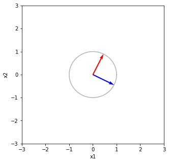
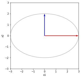
print("Vの列ベクトルと単位円")
plt.plot(uc[0,:], uc[1,:], color='black', alpha=0.3)
plt.quiver(0, 0, V[0, 0], V[0, 1], angles="xy", scale_units='xy', scale=1, color='red')
plt.quiver(0, 0, V[1, 0], V[1, 1], angles="xy", scale_units='xy', scale=1, color='blue')
plt.show()
x1 = np.dot(V, V.T)
c1 = np.dot(V, uc)
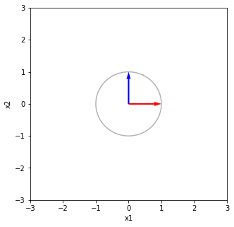
print("Vの列をV^Tで写像する V^TV 回転と鏡映")
print(x1)
plt.figure(figsize=(5, 5))
plt.xlim([-3, 3])
plt.ylim([-3, 3])
plt.xlabel('x1')
plt.ylabel('x2')
plt.plot(c1[0,:], c1[1,:], color='black', alpha=0.3)
plt.quiver(0, 0, x1[0, 0], x1[1, 0], angles="xy", scale_units='xy', scale=1, color='red')
plt.quiver(0, 0, x1[0, 1], x1[1, 1], angles="xy", scale_units='xy', scale=1, color='blue')
plt.show()
print("それをシグマで写像する ΣV^TV 軸方向に拡大・縮小(特異値倍)する")
x2 = np.dot(S2, x1 )
c2 = np.dot(S2, c1)
print(x2)
plt.figure(figsize=(5, 5))
plt.xlim([-3, 3])
plt.ylim([-3, 3])
plt.xlabel('x1')
plt.ylabel('x2')
plt.plot(c2[0,:], c2[1,:], color='black', alpha=0.3)
plt.quiver(0, 0, x2[0, 0], x2[1, 0], angles="xy", scale_units='xy', scale=1, color='red')
plt.quiver(0, 0, x2[0, 1], x2[1, 1], angles="xy", scale_units='xy', scale=1, color='blue')
plt.show()
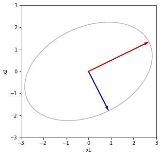
print("最後にUで写像する UΣV^TV 回転と鏡映")
print("u1とu2のσ1倍とσ2倍にそれぞれ重なる")
x3 = np.dot(U, x2)
c3 = np.dot(U, c2)
print(x3)
plt.figure(figsize=(5, 5))
plt.xlim([-3, 3])
plt.ylim([-3, 3])
plt.xlabel('x1')
plt.ylabel('x2')
plt.plot(c3[0,:], c3[1,:], color='black', alpha=0.3)
plt.quiver(0, 0, x3[0, 0], x3[1, 0], angles="xy", scale_units='xy', scale=1, color='red')
plt.quiver(0, 0, x3[0, 1], x3[1, 1], angles="xy", scale_units='xy', scale=1, color='blue')
plt.quiver(0, 0, S[0]*U[0, 0], S[0]*U[1, 0], angles="xy", scale_units='xy', scale=1, color='black', alpha=0.3)
plt.quiver(0, 0, S[1]*U[0, 1], S[1]*U[1, 1], angles="xy", scale_units='xy', scale=1, color='black', alpha=0.3)
plt.show()
特異値分解
U
[[ 0.89442719  0.4472136 ]
 [ 0.4472136  -0.89442719]]
S
[3. 2.]
V
[[ 0.4472136   0.89442719]
 [ 0.89442719 -0.4472136 ]]
USV^T
[[ 2.  2.]
 [-1.  2.]]
Vの列ベクトルと単位円
Vの列をV^Tで写像する V^TV 回転と鏡映
[[ 1.00000000e+00 -2.43158597e-17]
 [-2.43158597e-17  1.00000000e+00]]
それをシグマで写像する ΣV^TV 軸方向に拡大・縮小(特異値倍)する
 [[ 3.00000000e+00 -7.29475792e-17]
  [-4.86317195e-17  2.00000000e+00]]
最後にUで写像する UΣV^TV 回転と鏡映 u1とu2のσ1倍とσ2倍にそれぞれ重なる
 [[ 2.68328157  0.89442719]
  [ 1.34164079 -1.78885438]]

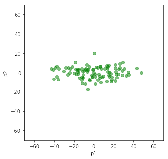
 の平均は
の平均は です.
です. に射影することを考えます.このとき,
 になります.射影の分散は
^2 = \mathbf u_1^T S \mathbf u_1") です.
です.(\mathbf x_i - \bar{\mathbf x})^T") です.
です. を
を の条件の下で最大化します.これはラグランジェの未定乗数法を用いて
")

 ですから,
ですから, の固有ベクトルです.
 をかけると
をかけると となり,データ
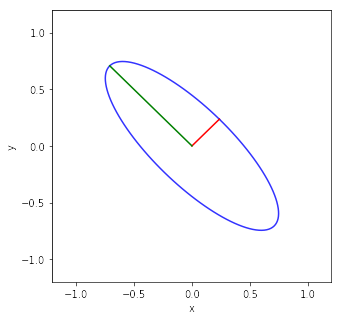
![\left[\begin{array}{cc}x & y\end{array}\right]\left[\begin{array}{cc}5 & 4\\ 4 & 5\end{array}\right]\left[\begin{array}{c}x\\ y\end{array}\right]=1](https://s0.wp.com/latex.php?latex=%5Cleft%5B%5Cbegin%7Barray%7D%7Bcc%7Dx+%26+y%5Cend%7Barray%7D%5Cright%5D%5Cleft%5B%5Cbegin%7Barray%7D%7Bcc%7D5+%26+4%5C%5C+4+%26+5%5Cend%7Barray%7D%5Cright%5D%5Cleft%5B%5Cbegin%7Barray%7D%7Bc%7Dx%5C%5C+y%5Cend%7Barray%7D%5Cright%5D%3D1&bg=ffffff&fg=000000&s=0 "\left[\begin{array}{cc}x & y\end{array}\right]\left[\begin{array}{cc}5 & 4\\ 4 & 5\end{array}\right]\left[\begin{array}{c}x\\ y\end{array}\right]=1")
 と置くと,
と置くと, を用いて
を用いて と表せる.行列
![[1\ 1]^T](https://s0.wp.com/latex.php?latex=%5B1%5C+1%5D%5ET&bg=ffffff&fg=000000&s=0 "[1\ 1]^T") である.固有値が1のとき固有ベクトルは
である.固有値が1のとき固有ベクトルは![[1\ -1]^T](https://s0.wp.com/latex.php?latex=%5B1%5C+-1%5D%5ET&bg=ffffff&fg=000000&s=0 "[1\ -1]^T") である.固有ベクトルの大きさは
である.固有ベクトルの大きさは であるので
であるので![\left[\begin{array}{cc}x & y\end{array}\right]\displaystyle\frac{1}{\sqrt{2}}\left[\begin{array}{rr}1 & 1\\ 1 & -1\end{array}\right]\left[\begin{array}{cc}9 & 0\\ 0 & 1\end{array}\right]\frac{1}{\sqrt{2}}\left[\begin{array}{rr}1 & 1\\ 1 & -1\end{array}\right]\left[\begin{array}{c}x\\ y\end{array}\right]=1](https://s0.wp.com/latex.php?latex=%5Cleft%5B%5Cbegin%7Barray%7D%7Bcc%7Dx+%26+y%5Cend%7Barray%7D%5Cright%5D%5Cdisplaystyle%5Cfrac%7B1%7D%7B%5Csqrt%7B2%7D%7D%5Cleft%5B%5Cbegin%7Barray%7D%7Brr%7D1+%26+1%5C%5C+1+%26+-1%5Cend%7Barray%7D%5Cright%5D%5Cleft%5B%5Cbegin%7Barray%7D%7Bcc%7D9+%26+0%5C%5C+0+%26+1%5Cend%7Barray%7D%5Cright%5D%5Cfrac%7B1%7D%7B%5Csqrt%7B2%7D%7D%5Cleft%5B%5Cbegin%7Barray%7D%7Brr%7D1+%26+1%5C%5C+1+%26+-1%5Cend%7Barray%7D%5Cright%5D%5Cleft%5B%5Cbegin%7Barray%7D%7Bc%7Dx%5C%5C+y%5Cend%7Barray%7D%5Cright%5D%3D1&bg=ffffff&fg=000000&s=0 "\left[\begin{array}{cc}x & y\end{array}\right]\displaystyle\frac{1}{\sqrt{2}}\left[\begin{array}{rr}1 & 1\\ 1 & -1\end{array}\right]\left[\begin{array}{cc}9 & 0\\ 0 & 1\end{array}\right]\frac{1}{\sqrt{2}}\left[\begin{array}{rr}1 & 1\\ 1 & -1\end{array}\right]\left[\begin{array}{c}x\\ y\end{array}\right]=1")
^2 + 1\left(\displaystyle\frac{x-y}{\sqrt{2}}\right)^2=1")
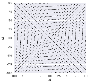
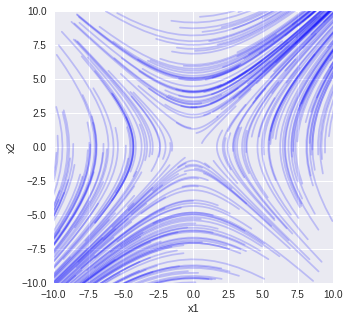
 と
と と置くと,
と置くと,
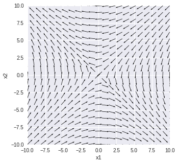
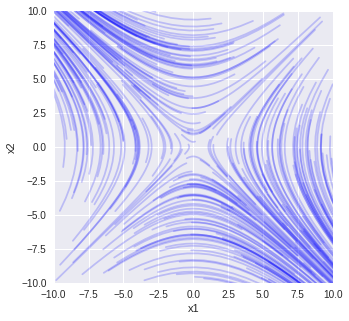
}{dt} = x_2(t)\\ \displaystyle\frac{dx_2(t)}{dt}=x_1(t)")
}{dt} = -x_2(t)\\ \displaystyle\frac{dx_2(t)}{dt}=-x_1(t)")